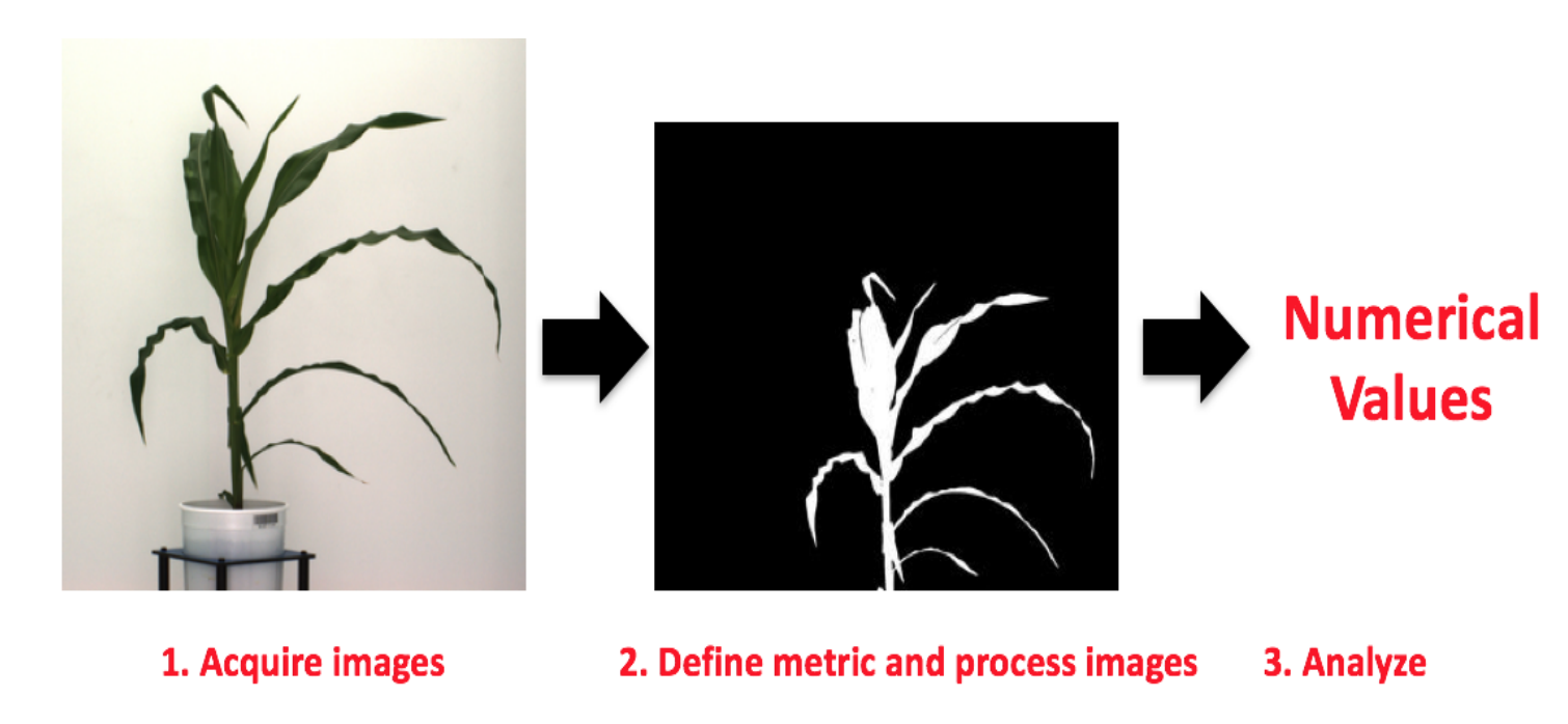
Statistical methods for the quantitative genetic analysis of high-throughput phenotyping data

class: center, middle, inverse, title-slide

# Statistical methods for the quantitative genetic analysis of high-throughput phenotyping data
## Factor analysis and network analysis to characterize high-dimensional phenotypic data <br /> The 64th RBras and 18th SEAGRO Meeting
### Gota Morota <br /><a href="http://morotalab.org/" class="uri">http://morotalab.org/</a> <br />
### 2019/8/2

---

# NSF funded project - wrchr.org 
![](hk1.png)

---
# NSF funded project - wrchr.org 
![](hk2.png)

---
# NSF funded project - wrchr.org 
<img src="hk4.png" height="506px" width="750px"/>

---
# High-throughput phenotyping
![](pheno.png)

---
# Pixelomics
![](pix.png)
Converting image data into numerical values (e.g., 12.5, 45.8, 25.9, etc.)

---
# Projected shoot area
<img src="PSA5.png" height="530px" width="600px"/>

---
# How to handle a large number of phenotypes?
More and more phenotypes are being generated across time and space
<img src="bigPhe.png" height="130px" width="600px"/>

Challenges:
- high dimensional phenotypes
- diverse phenotypes
- how to make sense of these data and interpret
-  multi-trait linear mixed model is computationally challenging

Objective:
- use Bayesian confirmatory factor analysis and Bayesian
- network to characterize a wide spectrum of rice phenotypes

---
# Bayesian confirmatory factor analysis
Assume observed phenotypes are derived from  underlying latent variables

`\begin{align*}
    \mathbf{T} =  \mathbf{\Lambda} \mathbf{F} + \mathbf{s}
\end{align*}`
  
- `\(\mathbf{T}\)` is the `\(t \times n\)` matrix of observed phenotypes (413 accessions)

- `\(\mathbf{\Lambda}\)` is the `\(t \times q\)` factor loading matrix

- `\(\mathbf{F}\)` is the `\(q \times n\)` latent variables matrix

- `\(\mathbf{s}\)` is the `\(t \times n\)` matrix of specific effects.

`\begin{align*}
    var\mathbf{(T)} &= \mathbf{\Lambda}\mathbf{\Phi}\mathbf{\Lambda}' + \mathbf{\Psi},
\end{align*}`

- `\(\mathbf{\Phi}\)` is the variance of latent variables

- `\(\mathbf{\Psi}\)` is the variance of specific effects

---
# Prior distributions

`\begin{align*}
    var\mathbf{(T)} &= \mathbf{\Lambda}\mathbf{\Phi}\mathbf{\Lambda}' + \mathbf{\Psi},
\end{align*}`

- Factor loading matrix: 
`\begin{align*}
& \mathbf{\Lambda} \sim \mathcal{N}(0, 0.01)
\end{align*}`

- Variance of latent variables:
`\begin{align*}
\mathbf{\Phi} \sim \mathcal{W}^{-1}(\mathbf{I}_{66}, 7) 
\end{align*}`

- Variance of specific effects:
`\begin{align*}
\mathbf{\Psi} \sim \Gamma^{-1} (1, 0.5)
\end{align*}`

---
# Define 6 latent variables from 48 phenotypes

1. Grain Morphology (Grm, 11)
    - Seed length (Sl), Seed width (Sw), Seed volume (Sv), etc
2. Morphology (Mrp, 14)
    - Flag leaf length (Fll), Flag leaf width (Flw), etc
3. Flowering Time (Flt, 7)
    - Flowering time in Arkansas (Fla), Flowering time in Aberdeen (Flb), etc}
4. Ionic components of salt stress (Iss, 6) 
    - Na shoot (Nas), K shoot salt (Kss), etc
5. Yield (Yid, 5)
    - Panicle number per plant (Pnu),   Panicle length (Pal), etc
6. Morphological salt response (Msr, 5)  
    - Shoot BM ratio (Sbr), Root BM ratio (Rbr), etc

---
# Study the genetics of each latent variable
<img src="BCFA.jpg" height="530px" width="700px"/>

---
# Multivariate analysis
Bayesian genomic best linear unbiased prediction
    - separate genetic effects from noise (44K SNPs)
    
`\begin{align*}
    \mathbf{F} = \boldsymbol{\mu} + \mathbf{Xb} + \mathbf{Zu} + \boldsymbol{\epsilon}
\end{align*}`

- `\(\mathbf{F}\)` : Vector of factor scores
- `\(\mathbf{X}\)` : Incidence matrix for fixed effects 
- `\(\mathbf{Z}\)` : Incidence matrix for additive genetic effects
- `\(\mathbf{b}\)`: Vector of fixed effects
- `\(\mathbf{u}\)`: Vector of additive genetic effects
- `\(\mathbf{e}\)`: Vector of residuals

---
# Piror distributions
`\begin{align*}
    \mathbf{F} = \boldsymbol{\mu} + \mathbf{Xb} + \mathbf{Zu} + \boldsymbol{\epsilon}
\end{align*}`

<div align="center">    
<img src="MTMvar.png" height="100px" width="500px"/>
</div>
- `\(\boldsymbol{\mu}\)` and `\(\mathbf{b}\)` were assigned a flat prior

- `\(\boldsymbol{\Sigma_{u}}\)`, `\(\boldsymbol{\Sigma_{e}}\)` are variance-covariance matrix between latent variables

`\begin{align*}
\boldsymbol{\Sigma_{u}}, \boldsymbol{\Sigma_{e}} \sim \mathcal{W}^{-1}(\mathbf{I}_{66}, 6) 
\end{align*}`

---
# Bayesian Network
Probabilistic directed acyclic graphical model
    - interrelationship (Edges) among latent variables (Nodes)
    - genetic selection for breeding requires causal assumptions

---
# Constraint-based learning
<img src="Fig3.jpg" height="530px" width="700px"/>

---
# Score-based learning
<img src="Score-based-diagram.png" height="500px" width="700px"/>

---
# Examples of algorithms
Score-based algorithm

- Hill climbing
- Tabu search

Hybrid algorithm

- Max-Min Hill Climbing algorithm
- General 2-Phase Restricted Maximization algorithm

---
# Standardized factor loadings
<img src="load2.png" height="506px" width="500px"/>

---
# Standardized factor loadings
<img src="load3.png" height="466px" width="500px"/>

---
# Genetic correlations among latent variables
<img src="Cor_plot_for_presentation.png" height="530px" width="700px"/>

---
# Hill Climbing algorithm
<img src="BN_HC.png" height="530px" width="700px"/>

---
# Tabu algorithm
<img src="BN_TABU.png" height="530px" width="700px"/>

---
# Max-Min Hill Climbing algorithm
<img src="BN_MMHC.png" height="530px" width="700px"/>

---
# General 2-Phase Restricted Maximization algorithm
<img src="BN_RSMAX2.png" height="460px" width="650px"/>

---
# Consensus Bayesian network
<img src="BN_consensus.png" height="460px" width="650px"/>

---
# Paper - 10.1534/g3.119.400154
<img src="G32018.png" height="460px" width="650px"/>

---
# FA vs. PCA

- What is the main difference between principal component analysis (PCA) and factor analysis (FA)?

---
# Confirmatory factor analysis vs. Explanatory factor analysis
<img src="CFAvsEFA.png" height="460px" width="650px"/>

---
# EFA analysis in wheat
<img src="CFAvsEFA.png" height="460px" width="650px"/>

---

---
# Summary

- Bayesian cofirmatory factor analysis allows to work at the
level of latent variables

- Bayesian network can be applied to predict the potential influence of external interventions or selection associated with target traits

- Provide greater insights than pairwise-association measures of multiple phenotypes

- It is possible to dissect genetic signals from high-dimensional phenotypes if we focus on underlying patterns in big data