class: center, middle, inverse, title-slide # Genetic analysis of time series phenomics ## Quantitative Genetics Short Course <span class="citation">@UFV</span> ### Gota Morota <br /><a href="http://morotalab.org/" class="uri">http://morotalab.org/</a> <br /> ### 2019/11/20 --- # High-throughput phenomics .pull-left[ <div align="left"> <iframe src="https://innovate.unl.edu/video/leasing-options/greenhouse-innovation-center.mp4" width="250" height="150" frameBorder="0" class="giphy-embed" allowFullScreen></iframe><p><a href="https://innovate.unl.edu/greenhouse-innovation-center">UNL Greenhouse Innovation Center</a> </p> </div> <div align="left"> <iframe width="260" height="200" src="https://www.youtube.com/embed/wor4BFjbIyI?rel=0" frameborder="0" allow="autoplay; encrypted-media" allowfullscreen></iframe> <p><a href="https://www.youtube.com/watch?v=wor4BFjbIyI">Spidercam</a> </div> ] .pull-right[ <div align="right"> <img src="https://www.frontiersin.org/files/Articles/254051/fpls-08-00421-HTML/image_m/fpls-08-00421-g002.jpg" width=400 height=400><p>Unmanned aerial vehicle<a href="https://www.frontiersin.org/articles/10.3389/fpls.2017.00421/full"> (Watanabe et al. 2017)</a> </div> ] --- # Pixelomics 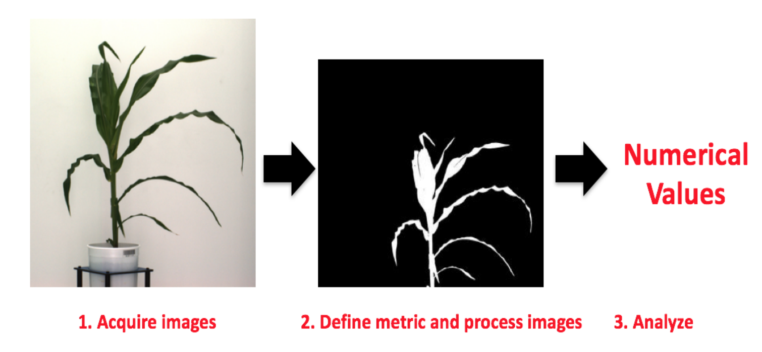 Converting image data into numerical values (e.g., 12.5, 45.8, 25.9, etc.) --- # Automated image-based phenomics facility 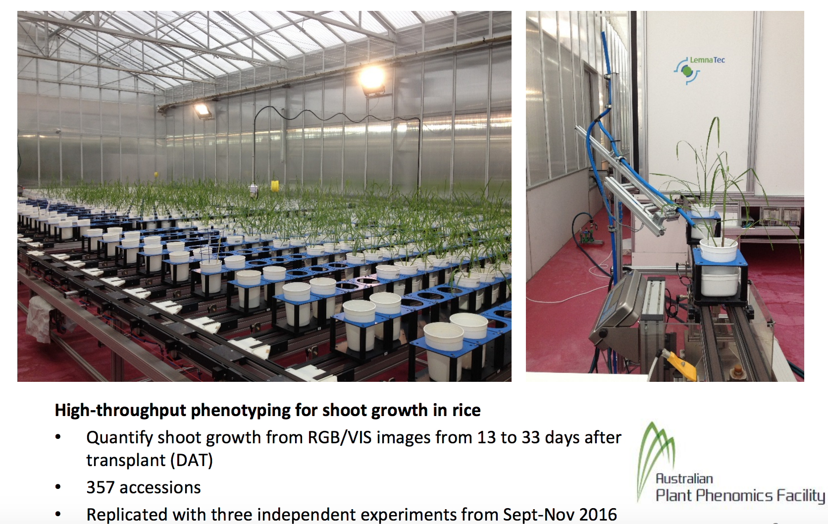 --- # Automated high-throughput phenotyping <iframe width="700" height="500" src="https://www.youtube.com/embed/JWNoQ3w-KbY" frameborder="0" allow="accelerometer; autoplay; encrypted-media; gyroscope; picture-in-picture" allowfullscreen></iframe> --- # Longitudinal data Projected shoot area (PSA) = the sum of plant pixel from two side-view images and one top-view <div align="center"> <img src="mackPSA.png" width=400 height=200><p><a href=""> Campbell et al. (2018)</a> </div> - Single time point analysis - cross-sectional analysis - Longitudinal analysis - leverage covariance among time points - account for longitudinal curve --- # Random regression model (RRM, longitudinal GBLUP) Predict random regression coefficients for each line using GBLUP `\begin{align*} \text{PSA}_{tjk} =\mu + \sum_{k=0}^{K_1}\phi(t)_{jk}\beta_k + \sum_{k=0}^{K_2}\phi(t)_{jk} u_{jk} + \sum_{k=0}^{K_3}\phi(t)_{jk} pe_{jk} + \epsilon_{tjk} \end{align*}` - `\(\beta_k\)`: fixed mean trajectory - `\(\phi\)`: Legendre polynomial - `\(u\)`: random additive genetic effect - `\(pe\)`: random permanent environmental effect - `\(K\)`: order of fit - `\(\epsilon\)` residual At time `\(t\)`, the GBLUP for the `\(j\)`th individual is `\begin{align*} \text{GBLUP}_{jt} = \phi_t\hat{u}_j \end{align*}` where `\(\phi_t\)` is the row vector of the matrix of Legendre polynomials. --- # Legendre polynomials <img src="LegExample.png" height="500px" width="550px"/> --- # The Phi matrix Suppose there are 20 time points (t `\(\in\)` 1, 2, `\(\cdots\)`, 20) $$ \boldsymbol{\Phi} = \mathbf{M} \boldsymbol{\Lambda} $$ - `\(\mathbf{M}\)` is the `\(t_{max}\)` by `\(d + 1\)` matrix containing the polynomials of the standardized time covariate `\(\mathbf{M}_{k+1} = \left ( \frac{2(t - t_{min} )}{t_{max} - t_{min}} \right )^k- 1\)` - `\(\boldsymbol{\Lambda}\)` is the `\(d + 1 \times d + 1\)` matrix of Legendre polynomial coefficients <img src="phi2.png" height="310px" width="350px"/> --- # Some examples - [http://morotalab.org/Mrode2005/rr/rr.html](http://morotalab.org/Mrode2005/rr/rr.html) --- # Matrix notation of RRM $$ \mathbf{y} = \mathbf{Xb} + \mathbf{Z}_1 \mathbf{u} + \mathbf{Z}_2 \mathbf{pe} + \boldsymbol{\epsilon} $$ - `\(\mathbf{y}\)`: a column vector of `\(n'\)` by 1, where `\(n'\)` is the number of records - `\(\mathbf{X}\)`: a matrix of `\(n'\)` by `\(K_1\)` - `\(\mathbf{Z_1}\)`: a matrix of `\(n'\)` by `\(n * K_2\)` - `\(\mathbf{Z_2}\)`: a matrix of `\(n'\)` by `\(n * K_3\)` 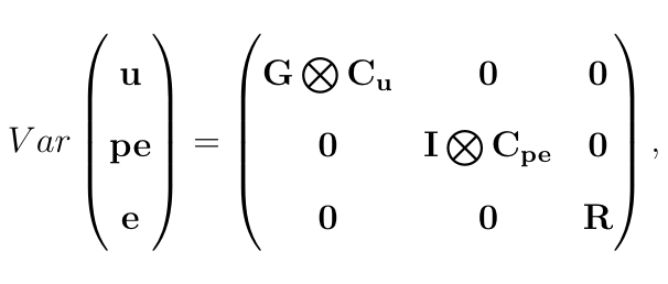 --- # Longitudinal genomic prediction <img src="mackCV.jpg" height="510px" width="450px"/> --- # Longitudinal genomic prediction <img src="mackCV2.jpg" height="400px" width="650px"/> --- # Longitudinal genomic prediction <img src="plantdirect.png" height="330px" width="650px"/> --- # Back-solving for SNP effects for shoot growth trajectories - Predict genetic values with random regression model - Solve for SNP effects `\begin{align*} BLUP(\boldsymbol{\beta}) &= \mathbf{W'}(\mathbf{WW'})^{-1}BLUP(\mathbf{g}). \end{align*}` Then standardization of SNP effect is given by ([Duarte et al. 2014](https://doi.org/10.1186/1471-2105-15-246)) `\begin{align*} \text{SNP}_{jt} &= \frac{ \mathbf{\hat{\beta}} }{ \sqrt{\text{Var}(\mathbf{\hat{\beta})}} } \\ p\text{-value}_{SNP_{jt}} &= 2(1 - \phi (|\text{SNP}_{jt}|)). \end{align*}` where `\begin{align*} \text{Var}(\boldsymbol{\hat{\beta}}) = \mathbf{W'G^{-1}W}\sigma^2_g - \mathbf{W'G^{-1}C^{22}G^{-1}W }\sigma^2_e. \end{align*}` --- # Variance of marker effect <img src="varB1.png" height="256px" width="650px"/> `\begin{align*} \textrm{Var(} \hat{\mathbf{u}} \textrm{)} &= \mathbf{G} \sigma^2_g - \mathbf{C^{22}} \sigma^2_e \end{align*}` Thus, `\begin{align*} \text{Var}(\boldsymbol{\hat{\beta}}) = \mathbf{W_{sc}'G^{-1}W_{sc}}\sigma^2_g - \mathbf{W_{sc}'G^{-1}C^{22}G^{-1}W_{sc} }\sigma^2_e. \end{align*}` --- # Variance of marker effect  - `\(\mathbf{C^{22}}\)` is `\(n * K_2 \times n * K_2\)` - `\(\boldsymbol{\Phi_{g}^*}\)` is a `\(n * t \times K_2 * n\)` block matrix where the diagonal sub-matrices consist of Legendre polynomials at each standardized time interval. - `\(\mathbf{C^{22*}}\)` is `\(n * t \times n * t\)` --- # Manhattan plots (700K SNPs) <img src="Fig2_alt.png" height="356px" width="650px"/> Top: random regression model. Bottom: single time point model --- # Persistent and time specific QTL signals 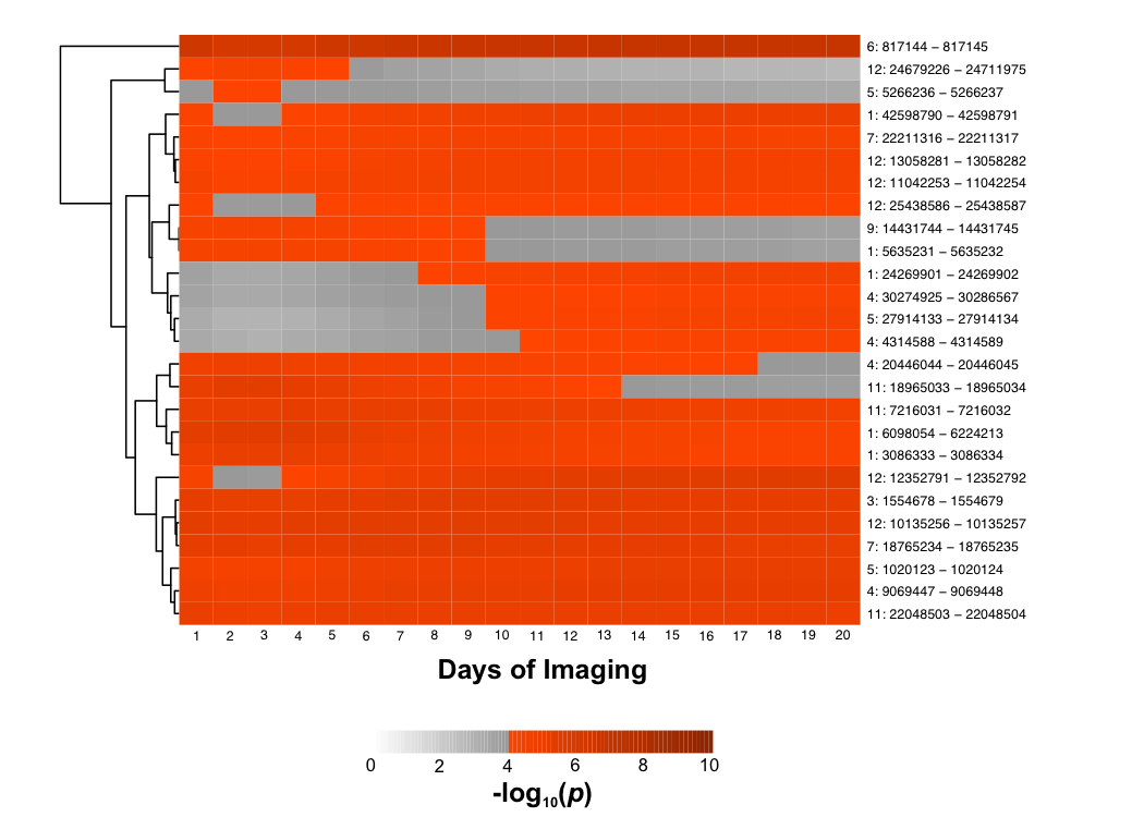 --- # Longitudinal GWAS  [https://doi.org/10.3835/plantgenome2018.10.0075](https://doi.org/10.3835/plantgenome2018.10.0075) --- # Projected shoot area  --- # Legendre polynomials vs. B-splines  --- # B-splines Given a preconsidered knot sequence of time `\(t\)`, the covariables for B-splines of degree `\(d = 0\)` were defined by assuming values of unity for all points in a given interval or zero otherwise. For the `\(i\)`th interval given by knots <img src="BsplineMath.png" height="300px" width="500px"/> The number of regression coefficients is given by the number of knots + degree − 1. --- # Longitudinal CV scenarios <img src="CV_Scenario.png" height="450px" width="650px"/> --- # Longitudinal CV scenarios * CV1: The time-specific genetic value of the `\(i\)`th individual in the training set was computed as `\(\hat{\mathbf{g}}_\text{trn, i}^{t} = \boldsymbol{\Phi}_t \mathbf{u}_{i}\)`, where `\(\hat{\mathbf{g}}_\text{trn, i}^{t}\)` is the estimated genetic value of the individual `\(i\)` at time `\(t\)`; `\(\boldsymbol{\Phi}_t\)` is the `\(t\)`th row vector of the `\(t_\text{max} \times K_1\)` matrix `\(\boldsymbol{\Phi}\)`; and `\(\mathbf{u}_i\)` is the `\(i\)`th column vector of the `\(K_1 \times n\)` matrix `\(\mathbf{u}\)`. Then, a vector of predicted genetic values of individuals in the testing set at time `\(t\)` was obtained as `\(\hat{\mathbf{g}}_\text{tst}^{t} = \mathbf{G}_{\text{tst, trn}} \mathbf{G}_{\text{trn, trn}}^{-1} \hat{\mathbf{g}}_\text{trn}^{t}\)`, where `\(\mathbf{G}_{\text{tst, trn}}\)` is the genomic relationship matrix between the testing and training set and `\(\mathbf{G}_{\text{trn, trn}}^{-1}\)` is the inverse of genomic relationship matrix between the training set. * CV2 and CV3: First estimate the random regression coefficient matrix `\(\mathbf{u}\)` using `\(\boldsymbol{\Phi}_{1:t}\)`, which was computed from time point 1 to time point `\(t\)`. The prediction of future time points `\(t'\)` ( `\(t+1 \leq t' \leq t_\text{max}\)` ) for an individual `\(i\)` was carried out by `\(\hat{\mathbf{g}}^{t'} = \boldsymbol{\Phi}_{t'} \mathbf{u}_{i}\)`, where `\(\boldsymbol{\Phi}_{t'}\)` is the `\(t^{'}\)`th row vector of `\(t_\text{max} - t\)` by `\(K + 1\)` matrix `\(\boldsymbol{\Phi}\)`; and `\(\mathbf{u}_i\)` is the `\(i\)`th column vector of the number of random regression coefficients by `\(n\)` matrix `\(\mathbf{u}\)`. --- # CV1 - RRM vs. MTM  --- # CV2 control conditions 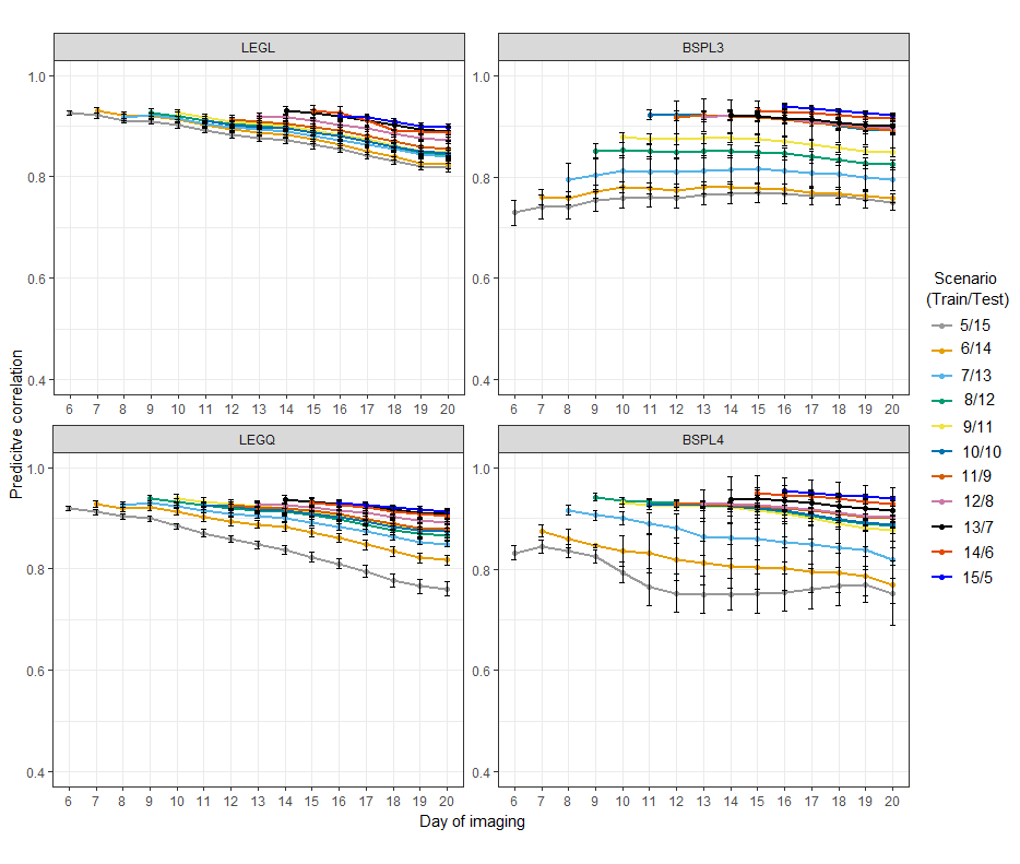 --- # CV2 stress conditions 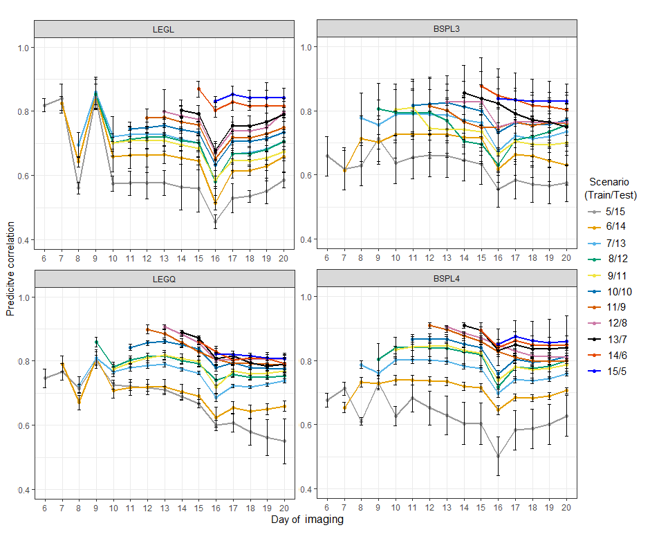 --- # CV3 control conditions 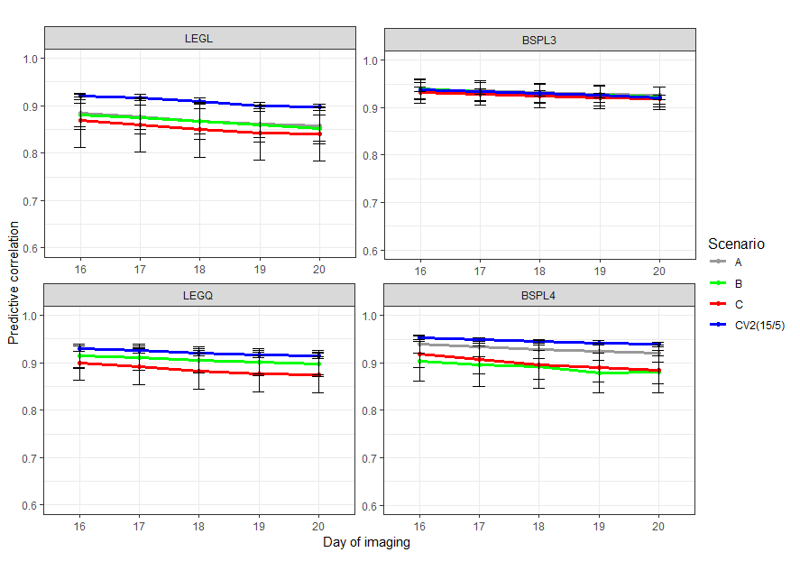 --- # CV3 stress conditions 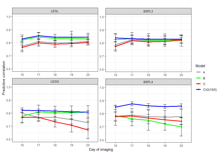 --- # Goodness-of-fit vs. Prediction 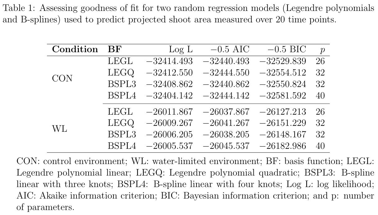 --- # bioRxiv preprint 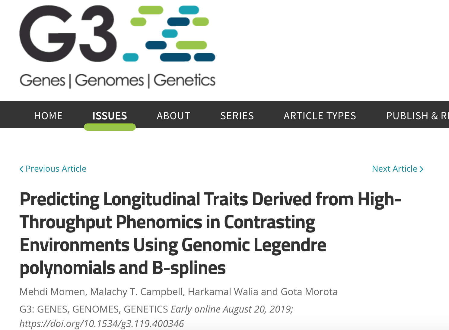 [doi: https://doi.org/10.1101/632117](https://doi.org/10.1101/632117) --- # Additional topics 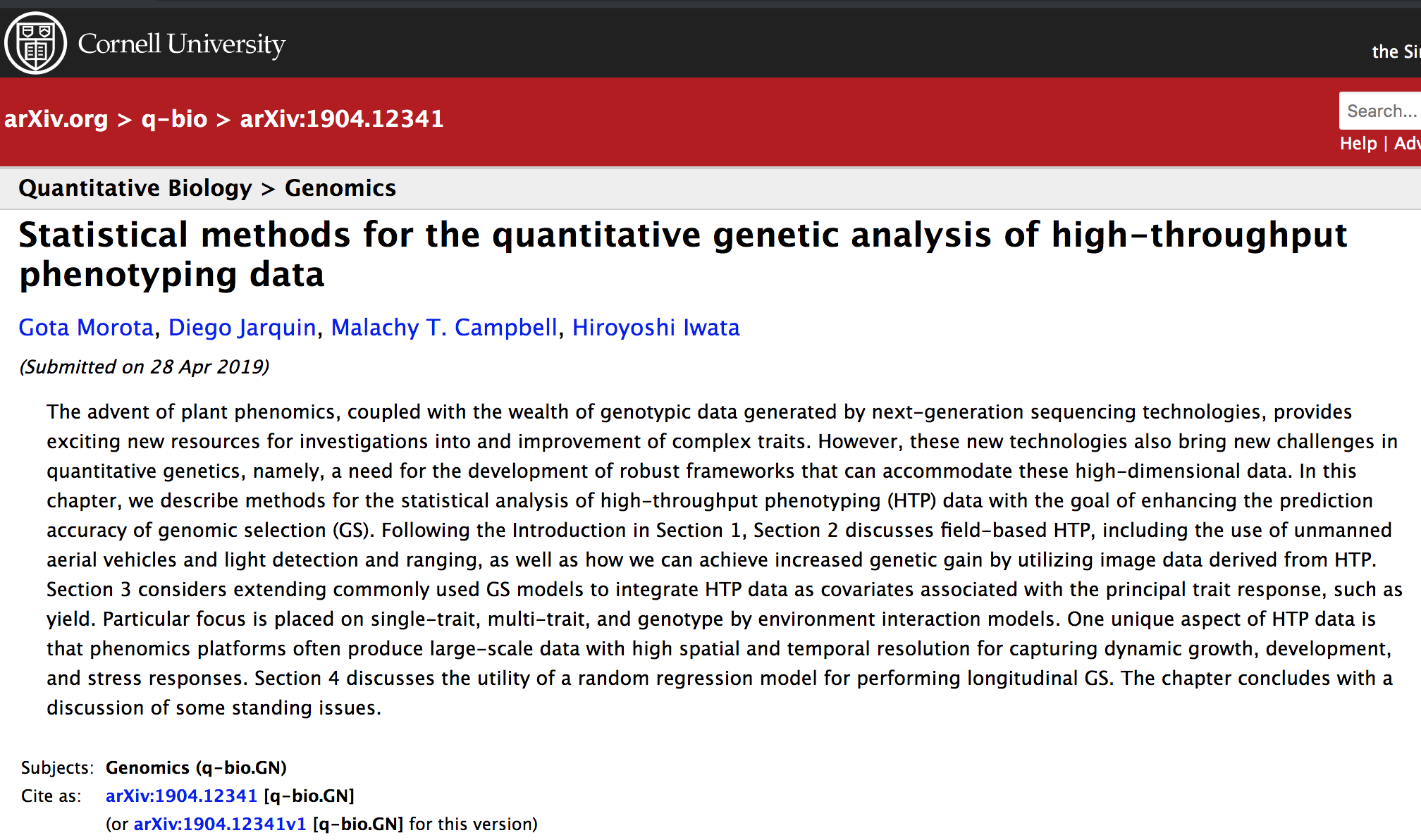 [https://arxiv.org/abs/1904.12341](https://arxiv.org/abs/1904.12341) --- # Software - [ASReml](https://www.vsni.co.uk/software/asreml/) - [Wombat](http://didgeridoo.une.edu.au/km/wombat.php) - [BLUPF90](http://nce.ads.uga.edu/wiki/doku.php) --- # Summary - Random regression models provide a flexible framework for longitudinal genomic prediction and longitudinal GWAS - Greater prediction accuracy with random regression - Identifies time-specific genetic signals - Deep learning?