Variance heterogeneity analysis

class: center, middle, inverse, title-slide

# Variance heterogeneity analysis
## Quantitative Genetics Short Course <span class="citation">@UFV</span>
### Gota Morota <br /><a href="http://morotalab.org/" class="uri">http://morotalab.org/</a> <br />
### 2019/11/26

---

# Epistasis what is it?
![](Cordell.png)

---
# How to parameterize response variable `$\mathbf{y}$` ?
Example: 50,000 SNP panel

- additive model 
    - 50K effects to estimate
- additive + dominance model 
    - 50K + 50K effects to estimate!
- additive + dominance  + second-order epistasis model 
    - 50K + 50K RV + `${50\text{K} \choose 2}$` effects to estimate

1. Overparameterization!!!!!

2. Curse of dimensionality

---
# Mean heterogeneity analysis
- mean value difference between genotypes
- average effect of allele substitution
- standard GWAS is designed to capture these genetic signals

---
# Variance heterogeneity analysis
- heterogenity of variance between genotypes
- variance heterogeneity loci (vQTL) or variance GWAS
(vGWAS)
- standard GWAS is not able to capture these genetic signals

---
# Example: Variance heterogeneity locus
<img src="varQTL.png" height="406px" width="650px"/>

---
# Variance heterogeneity loci
Variance heterogeneity loci are potentially involved in
- buffer the impact of cryptic genetic variations
- release of hidden genetic variation
- developmental stability
- phenotypic plasticity

.pull-left[
<img src="LynchWalsh.jpg" height="256px" width="250px"/>
]

.pull-right[
<img src="WalshLynch.jpg" height="256px" width="250px"/>
]

Epistasis

---
# Non-epistatic variance QTL vs. Epistatic variance QTL 
<img src="PGRP.png" height="406px" width="650px"/>

---
# Association mapping panel
- hard winter wheat association panel of 299 lines
- cadmium concentration
- 90,000 markers (Wang et al. 2014)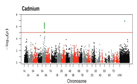

![Guittieri et al., 2015](Guittieri2015.png)

Guittieri et al., 2015

---
# Double generalized linear model (DGLM)
$$
`\begin{align}
  \mathbf{y} &= \mathbf{1}\mu_m + \mathbf{X}\mathbf{b} +  \mathbf{S}_m a_m + \boldsymbol{\epsilon} \\
   \boldsymbol{\epsilon}_i  \sim& N(0, \sigma^{2}_{\epsilon_i}) \\\
    \log  (\sigma^2_{\epsilon_i}) &=   \mathbf{1}\mu_v + \mathbf{S}_v a_v. 
\end{align}`
$$
- `$\sigma^2_{\epsilon_{i}} \sim \frac{ \hat{\epsilon}_i^2 }{ 1 - h_{ii}}$` is fitted using  GLM of a gamma distribution with a log link function, where weights are provided by `$\frac{1 - h_{ii}}{2}$` and a linear predictor equals to a single marker covariate `$\mathbf{s}\mathbf{a}$`.

- equivalent to modeling  `$\mathbf{y} \sim N(\mathbf{1}\mu_m + \mathbf{X}\mathbf{b} + \mathbf{S}_m a_m, \exp(\mathbf{1}\mu_v + \mathbf{S}_va_v) )$`

- works in an iterative manner between the mean and variance parts of the model

---
# Hierarchical generalized linear model (HGLM)
$$
`\begin{align}
  \mathbf{y} &= \mathbf{1}\mu_m + \mathbf{X}\mathbf{b} +  \mathbf{S}_m a_m +  \mathbf{Z}\mathbf{u} + \boldsymbol{\epsilon} 
\end{align}`
$$

- `$\mathbf{u} \sim N(0, G \sigma^2_g)$` is assumed to be a stochastic Gaussian process with mean zero and covariance function defined by a genomic relationship matrix `$\mathbf{G}$`

Variance GWAS
- equivalent to peforming vGWAS after adjusting for  potential covariates and mean-controlling effect

---
# Epistasis analysis
Pairwise interaction analyses for significant variance heterogenity markers 
$$
`\begin{align*}
\mathbf{y} &= \mathbf{1}\mu +  \mathbf{X}\mathbf{b} +  \mathbf{S}_j\mathbf{a}_j + \mathbf{S}_k\mathbf{a}_k + ( \mathbf{S}_j \mathbf{S}_k)\nu_{jk} + \boldsymbol{\epsilon}
\end{align*}`
$$

- `$\mathbf{X}$` is the incident matrix for the first four PCs

- `$S_j$` and `$S_k$` are SNP codes for the jth and kth markers

---
# Results: Mean and variance GWAS
<img src="circle1.png" height="506px" width="600px"/>

---
# Results: Variance GWAS loci
<img src="violin1.png" height="506px" width="600px"/>

---
# Results: Epistasis analysis
<img src="epi1.png" height="506px" width="600px"/>

---
# Preprint
![](bioRxiv.png)

---
# Morota lab at Virginia Tech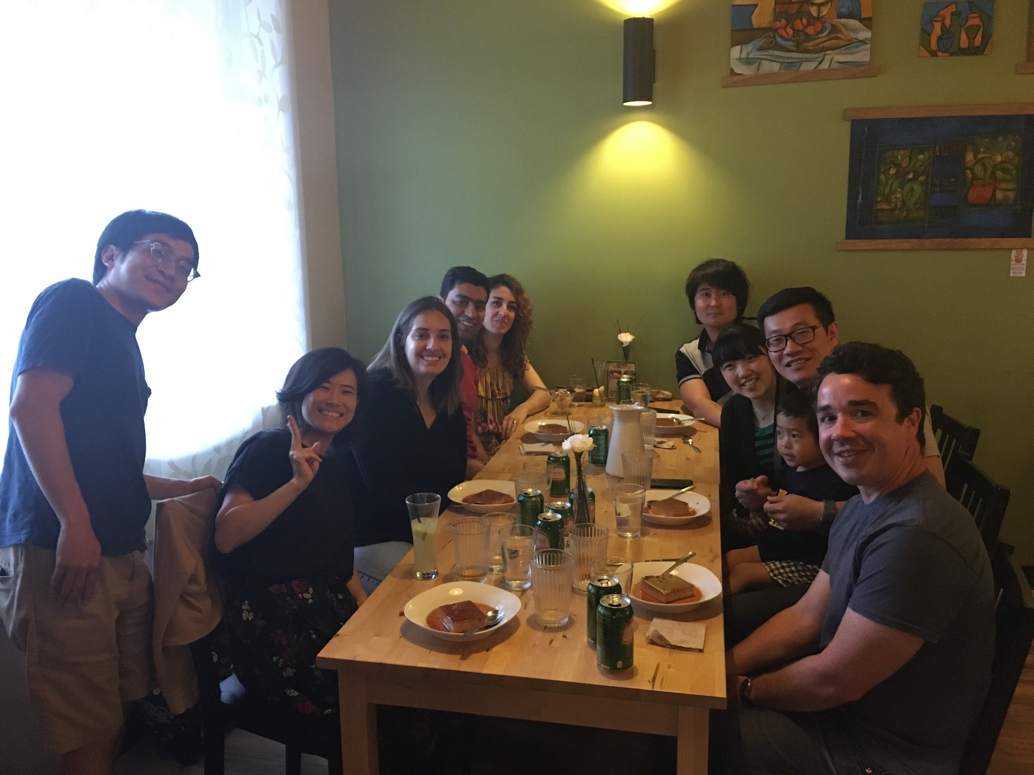
![](SabrinaParty.jpg)
<img src="SabrinaParty.jpg" height="506px" width="600px"/>