class: center, middle, inverse, title-slide # Introduction to Quantitative Genetics ## Statistical Methods for Omics-assisted Breeding Hands-on Workshop ### Gota Morota <br /><a href="http://morotalab.org/" class="uri">http://morotalab.org/</a> <br /> ### 2018/11/12 --- # About me  --- class: inverse, center, middle # Quantitative Genetics -- Analysis of complex or multifactorial traits -- All genes affect all traits - the question is by how much? -- Infinitesimal model -- Oligogenic model --- # What is quantitative genetics? -- Population genetics - **Mathematics** is language of population genetics, **population genetics** is language of **evolution**. -- Quantitative genetics - **Statistics** is language of quantitative genetics, **quantitative genetics** is language of **complex trait genetics**. -- **Phenotypes** first in quantitative genetics In the era of genomics, phenotype is **king** --- # Regression model Galton (1886). Regression towards mediocrity in hereditary stature "<img src="galton1886.png" width=600 height=380> --- # Complex traits "<img src="phenotype-plant.png" width=800 height=530> --- # Genetic values Quantitative genetic model: `\begin{align*} \mathbf{y} &= \mathbf{g} + \boldsymbol{\epsilon} \\ \end{align*}` where `\(\mathbf{y}\)` is the vector of observed phenotypes, `\(\mathbf{g}\)` is the vector of genetic values, and `\(\boldsymbol{\epsilon}\)` is the vector of residuals. Example: | Plant ID | y | g | e | | ------------- |:-------------:| -----:|------| | 1 | 10 | ? | ? | | 2 | 7 | ? | ? | | 3 | 12 | ? | ? | --- # Genetic values Quantitative genetic model: `\begin{align*} \mathbf{y} &= \mathbf{g} + \boldsymbol{\epsilon} \\ \end{align*}` where `\(\mathbf{y}\)` is the vector of observed phenotypes, `\(\mathbf{g}\)` is the vector of genetic values, and `\(\boldsymbol{\epsilon}\)` is the vector of residuals. Example: | Plant ID | y | g | e | | ------------- |:-------------:| -----:|------| | 1 | 10 | 5 | 5 | | 2 | 7 | 6 | 1 | | 3 | 12 | 2 | 10 | -- Phenotypes can be observed and measured but genotypic and additive genetic effects cannot --- # Conventional Phenotyping 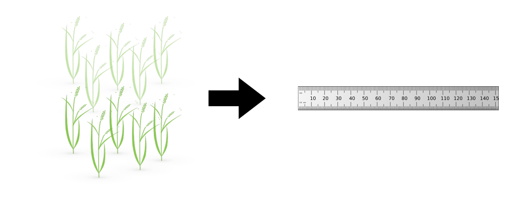 - labor intensive - prone to measurement error --- # Genomic information (e.g., SNPs) 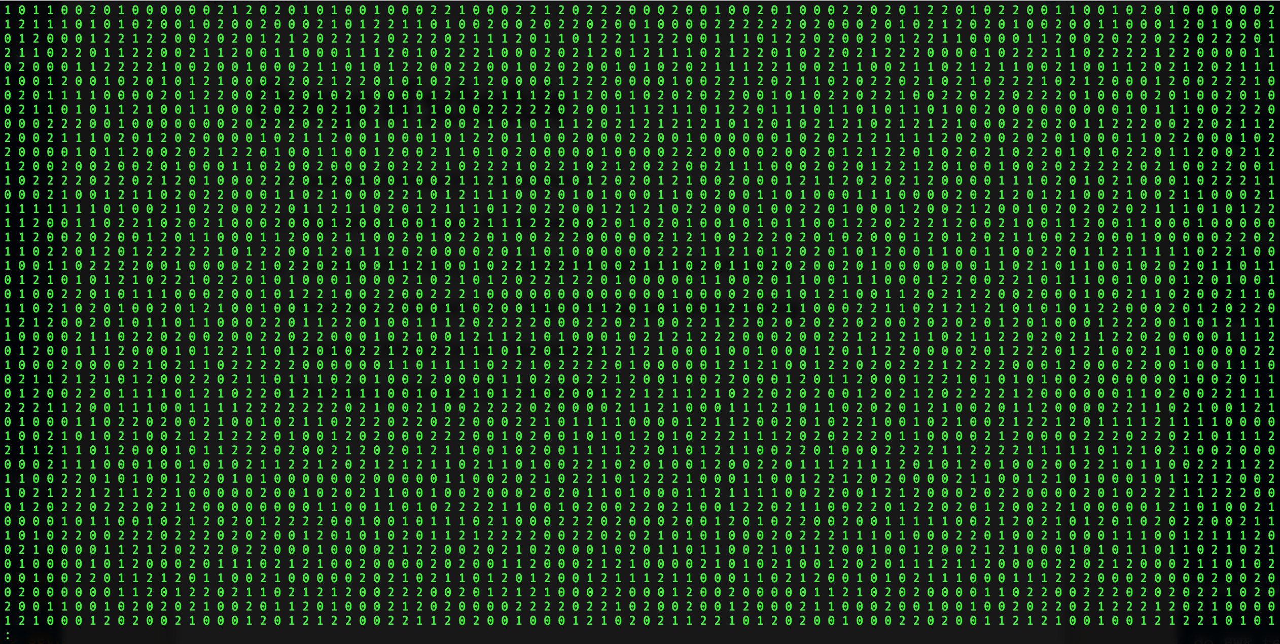 .center[Repeat of numbers 0, 1, and 2] --- # Quantitative genetics Connecting phenotypic data with genomic information<center> <div> <img src="plant.png" width=200 height=100> = <img src="SNPs.png" width=200 height=100> + error </div> </center> `\begin{align*} \mathbf{y} &= \mathbf{g} + \boldsymbol{\epsilon} \\ &\approx \mathbf{W}\mathbf{a} + \boldsymbol{\epsilon} \end{align*}` We approximate unknown `\(\mathbf{g}\)` with `\(\mathbf{Wa}\)`. `\begin{align*} \underbrace{\begin{bmatrix} y_1\\ y_2\\ \vdots \\ y_n\end{bmatrix}}_{n \times 1} &= \underbrace{\begin{bmatrix} w_{11} & w_{12} & \cdots & w_{1m} \\ w_{21} & w_{22} & \cdots & w_{2m} \\ \vdots & \vdots & \ddots & \vdots \\ w_{n1} & w_{n2} & \cdots & w_{nm} \end{bmatrix}}_{n \times m} \quad \underbrace{\begin{bmatrix} a_1\\ a_2\\ \vdots \\ a_m\end{bmatrix}}_{m \times 1} +\underbrace{\begin{bmatrix} \epsilon_1\\ \epsilon_2\\ \vdots \\ \epsilon_m\end{bmatrix}}_{n \times 1} \end{align*}` where `\(n\)` is the number of individuals (e.g., accessions) and `\(m\)` is the number of SNPs. --- # Precision agriculture using advanced technologies 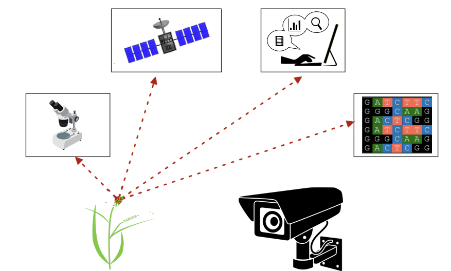 --- # Precision (digital) phenotyping  - automated process - less labor intensive - less prone to measurement error --- # Image phenotypes  &nbsp; &nbsp;  .center[Image data] [Phenotype is king!]() --- # Quantitative genetics Connecting image data with genomic information <center> <div> <img src="plant_01.png" width=100 height=100> = <img src="SNPs.png" width=100 height=100> + error </div> </center> `\begin{align*} \mathbf{y} &= \mathbf{g} + \boldsymbol{\epsilon} \\ &\approx \mathbf{W}\mathbf{a} + \boldsymbol{\epsilon} \end{align*}` We approximate unknown `\(\mathbf{g}\)` with `\(\mathbf{Wa}\)`. `\begin{align*} \underbrace{\begin{bmatrix} y_1\\ y_2\\ \vdots \\ y_n\end{bmatrix}}_{n \times 1} &= \underbrace{\begin{bmatrix} w_{11} & w_{12} & \cdots & w_{1m} \\ w_{21} & w_{22} & \cdots & w_{2m} \\ \vdots & \vdots & \ddots & \vdots \\ w_{n1} & w_{n2} & \cdots & w_{nm} \end{bmatrix}}_{n \times m} \quad \underbrace{\begin{bmatrix} a_1\\ a_2\\ \vdots \\ a_m\end{bmatrix}}_{m \times 1} +\underbrace{\begin{bmatrix} \epsilon_1\\ \epsilon_2\\ \vdots \\ \epsilon_m\end{bmatrix}}_{n \times 1} \end{align*}` where `\(n\)` is the number of individuals (e.g., accessions) and `\(m\)` is the number of SNPs. --- # Google Trends: 2012-2017  --- # Big and messy data Big data are being generated in almost every field - too large to permit visual inspection - big data `\(\ne\)` clean data - missing observations - empty cells - confounding - outliers --- # Big in n or m?  - `\(n\)`: number of individuals (records) - `\(m\)` number of SNPs (genetic markers) --- # Why we use big data in genetics? ([Makowsky et al., 2011](https://doi.org/10.1371/journal.pgen.1002051)) "<img src="makowsky1.png" width=700 height=400> --- # Why we use big data in genetics? ([Erbe et al., 2013](https://doi.org/10.1371/journal.pone.0081046)) "<img src="Erbe.png" width=700 height=400> --- # How to parameterize response variable y? - Prediction of additive genetic effects - `\(\mathbf{ y = S + a + \boldsymbol{\epsilon}}\)` - Prediction of total genetic effects **parametrically** - `\(\mathbf{ y = \mathbf{S} + \underbrace{\mathbf{ a + d + a*a + a*d + d*d}}_{g} + } \boldsymbol{\epsilon}\)` - Prediction of total genetic effects **non-parametrically** - `\(\mathbf{ y = \mathbf{S} + \mathbf{g} + \boldsymbol{\epsilon}}\)` --- # Prediction vs. Inference Complex traits are controlled by large number of genes with small effects, and influenced by both genetics and environments - Inference (location) - average effects of allele substitution - Inference (variability) - variance component estimation - genomic heritability Combination of above two (e.g., estimate proportion of additive genetic variance explained by QTLs) - Prediction - genomic selection - prediction of yet-to-be observed phenotypes --- # Prediction vs. Inference <div align="center"> <img src="Lo2015PNAS.png" width=900 height=400> </div> * [http://www.pnas.org/content/112/45/13892.abstract ](http://www.pnas.org/content/112/45/13892.abstract ) --- # Expectation and variance (1) Define the random variable `\(w\)` which takes the value 1 if in gametes, `\(A\)` is present at locus `\(A\)` and zero otherwise. `\begin{align*} w &= \begin{cases} 1 & \text{if gamete carries } A \text{ with frequency } p\\ 0 & \text{otherwise, i.e., } a \text{ with frequency } 1-p \end{cases} \\ \end{align*}` where `\(p\)` is the allele frequency of `\(A\)`. -- Then, `\begin{align*} E(x) &= p \times 1 + (1-p) \times 0 \\ &= p \\ E(x^2) &= p \times 1^2 + (1-p) \times 0^2 \\ &= p \end{align*}` Thus, the variance of allelic content is `\begin{align*} Var(x) &= E(x^2) - E(x)^2 \\ &= p - p^2 \\ &= p(1-p) \\ \end{align*}` --- # Expectation and variance (2) Define the random variable `\(W\)` which counts the number of reference allele `\(A\)`. `\begin{align*} W &= \begin{cases} 2 & \text{if } AA \text{ with frequency } p^2 \\ 1 & \text{if } Aa \text{ with frequency } 2p(1-p) \\ 0 & \text{if } aa \text{ with frequency } (1-p)^2 \end{cases} \\ \end{align*}` where `\(p\)` is the allele frequency of `\(A\)`. -- Then, `\begin{align*} E[W] &= 0 \times (1 - p_j)^2 + 1 \times [2p(1-p)] + 2 \times p^2 \\ &= 2p \\ E[W^2] &= 0^2 \times (1 - p_j)^2 + 1^2 \times [2p(1-p)] + 2^2 \times p^2 \\ &= 2p(1-p) + 4p^2 \\ \end{align*}` Thus, the variance of allelic counts is `\begin{align*} Var(W) &= E[W^2] - E[W]^2 \\ &= 2p(1-p) + 4p^2 - 4p^2\\ &= 2p(1-p) \end{align*}` --- # Alternative coding Define the random variable `\(W\)` which counts the number of reference allele `\(A\)`. `\begin{align*} W &= \begin{cases} 1 & \text{if } AA \text{ with frequency } p^2 \\ 0 & \text{if } Aa \text{ with frequency } 2p(1-p) \\ -1 & \text{if } aa \text{ with frequency } (1-p)^2 \end{cases} \\ \end{align*}` where `\(p\)` is the allele frequency of `\(A\)`. -- Then, `\begin{align*} E[W] &= -1 \times (1 - p_j)^2 + 0 \times [2p(1-p)] + 1 \times p^2 \\ &= −(1 − 2p + p^2) + p^2 = 2p-1 \\ E[W^2] &= (-1)^2 \times (1 - p_j)^2 + 0^2 \times [2p(1-p)] + 1^2 \times p^2 \\ &= 1 − 2p + p^2 +p^2 = 2p^2 − 2p + 1 \\ \end{align*}` Thus, the variance of allelic counts is `\begin{align*} Var(W) &= E[W^2] - E[W]^2 \\ &= 2p^2 − 2p + 1 − (4p^2 − 4p + 1)\\ &= -2p^2 + 2p = 2p(1-p) \end{align*}` --- # Centered marker codes `\begin{align*} W - E(W) &= \begin{cases} 2 -2p & \text{if } AA \text{ with frequency } p^2 \\ 1 - 2p & \text{if } Aa \text{ with frequency } 2p(1-p) \\ 0 - 2p & \text{if } aa \text{ with frequency } (1-p)^2 \end{cases} \\ \end{align*}` `\begin{align*} W - E(W) &= \begin{cases} 1 - (2p-1) = 2 -2p& \text{if } AA \text{ with frequency } p^2 \\ 0 - (2p-1) = 1 - 2p & \text{if } Aa \text{ with frequency } 2p(1-p) \\ -1 - (2p-1) = 0 - 2p & \text{if } aa \text{ with frequency } (1-p)^2 \end{cases} \\ \end{align*}` where `\(p\)` is the allele frequency of `\(A\)`. Therefore, the variance and the centered codes are the same. --- # Covariance `\begin{align*} w_{A} &= \begin{cases} 1 & \text{if gamete carries } A \text{ with frequency } p_A\\ 0 & \text{otherwise, i.e., } a \text{ with frequency } 1-p_A \end{cases} \\ w_{B} &= \begin{cases} 1 & \text{if gamete carries } B \text{ with frequency } p_B\\ 0 & \text{otherwise, i.e., } b \text{ with frequency } 1-p_B \end{cases} \end{align*}` -- `\begin{align*} E(w_A) &= p_A \\ Var(w_A) &= p_A(1-p_A) \\ E(w_B) &= p_B \\ Var(w_B) &= p_B(1-p_B) \\ E(w_A w_B) &= p_{AB} \\ Cov(w_A, w_B) &= D_{AB} = p_{AB} - p_{A}p_{B} \end{align*}` -- The quantity `\(D_{AB}\)` is defined to be the (gametic) linkage disequilibrium between alleles `\(A\)` and `\(B\)`. `\begin{align*} \rho_{AB} = cor(x_{A}, x_{B}) &= \frac{D_{AB}}{\sqrt{p_A(1-p_A)p_B(1-p_B)}} \\ r^2_{AB} &= \frac{D^2_{AB}}{p_A(1-p_A)p_B(1-p_B)} \end{align*}` --- class: inverse, center, middle # Curse of dimensionality --- # Ordinary least squares (OLS) Quantitative genetic model: `\(\mathbf{y} = \mathbf{Wa} + \boldsymbol{\epsilon}\)` How to find the SNP effects ( `\(\mathbf{a}\)` )? -- We minimize the residual sum of squares `\begin{align*} \boldsymbol{\epsilon}' \boldsymbol{\epsilon} &= (\mathbf{y-Wa})'(\mathbf{y-Wa}) \\ &= \mathbf{y}'\mathbf{y} - \mathbf{y}'\mathbf{W} \mathbf{a}- \mathbf{a}'\mathbf{W}'\mathbf{y} + \mathbf{a}'\mathbf{W}'\mathbf{W}\mathbf{a} \\ &= \mathbf{y}'\mathbf{y} - 2\mathbf{a}'\mathbf{W}'\mathbf{y} + \mathbf{a}'\mathbf{W}'\mathbf{W}\mathbf{a} \end{align*}` We take a partial derivative with respect to `\(\mathbf{a}\)` `\begin{align*} \frac{\partial \boldsymbol{\epsilon\epsilon}'}{\partial \boldsymbol{a}} &= 2 \mathbf{W}'\mathbf{W} \mathbf{a} - 2\mathbf{X}'\mathbf{y} \end{align*}` By setting the equation equal to zero, we obtain a least square estimator of `\(\mathbf{a}\)`. `\begin{align*} \mathbf{W}'\mathbf{W} \mathbf{a} &= \mathbf{W}' \mathbf{y} \\ \hat{\mathbf{a}} &= (\mathbf{W}'\mathbf{W})^{-1} \mathbf{W}' \mathbf{y} \end{align*}` --- # Ordinary least squares (OLS) - `\(\hat{\mathbf{a}}\)` is the vector of regression coefficient for markers, i.e., effect size of SNPs - if the Gauss-Markov theorem is met, `\(E[\hat{\mathbf{a}}] = \mathbf{a} \rightarrow\)` BLUE - `\(E[\boldsymbol{\epsilon}] = 0\)`, `\(Var[\boldsymbol{\epsilon}] = \mathbf{I}\sigma^2_{\epsilon}\)` What if number of SNPs ( `\(m\)` ) `\(>>\)` number of individuals ( `\(n\)` ) ??? -- - `\((\mathbf{W}'\mathbf{W})^{-1}\)` does not exist - Effective degrees of freedom --- # OLS: Single marker regression Test each marker for the presence of QTLs and select those with significant effects Problems: marker effect sizes are exaggerated Suppose the true model is given by two causal SNPs `\begin{align*} \mathbf{y} & = \mathbf{w}_1a_1 + \mathbf{w}_2a_2 + \boldsymbol{\epsilon} \\ \mathbf{y} & = \begin{smallmatrix} \underbrace{\mathbf{W}}_{n \times 2}\underbrace{\mathbf{a}}_{2 \times 1} \end{smallmatrix} + \boldsymbol{\epsilon} \end{align*}` The OLS estimator for the full mdoel is `\begin{align*} \begin{bmatrix} \hat{a}_1 \\ \hat{a}_2 \end{bmatrix} &= \begin{bmatrix} \mathbf{w}'_1\mathbf{w}_1 & \mathbf{w}'_1\mathbf{w}_2 \\ \mathbf{w}'_2\mathbf{w}_1 & \mathbf{w}'_2\mathbf{w}_2 \end{bmatrix}^{-1} \begin{bmatrix} \mathbf{w}'_1\mathbf{y} \\ \mathbf{w}'_2\mathbf{y} \\ \end{bmatrix} \\ \hat{\mathbf{a}} &= (\mathbf{W'W})^{-1}\mathbf{W}'\mathbf{y} \end{align*}` --- # OLS: Single marker regression The expectation of `\(\hat{\mathbf{a}}\)` is `\begin{align*} E(\hat{\mathbf{a}} | \mathbf{W}) = (\mathbf{W'W})^{-1}\mathbf{W'}E(\mathbf{y} ) = (\mathbf{W'W})^{-1}\mathbf{W'Wa} = \mathbf{a} \end{align*}` which is a nice property of BLUE. Now, what if we fit a single SNP model `\(\mathbf{y} = \mathbf{w}_1a_1 + \boldsymbol{\epsilon}\)`? The OLS estimate is `\(\hat{a}_1 = (\mathbf{w'_1w_1})^{-1}\mathbf{w}'_1\mathbf{y}\)` The expectation of `\(\hat{a}_1\)` is `\begin{align*} E(\hat{a}_1 | \mathbf{w}_1) &= (\mathbf{w'_1w_1})^{-1}\mathbf{w}'_1E(\mathbf{y}) \\ &= (\mathbf{w'_1w_1})^{-1}\mathbf{w'_1}[\mathbf{w_1a_1 + w_2a_2}] \\ &= \mathbf{(w'_1w_1)}^{-1}\mathbf{w'_1w_1}a_1 + (\mathbf{w'_1w_1})^{-1}\mathbf{w'_1w_2}a_2 \\ &= a_1 + (\mathbf{w'_1w_1})^{-1}\mathbf{w'_1w_2}a_2 \end{align*}` - OLS is biased if full model holds but fit a misspecified model - this bias is proportional to `\((\mathbf{w'_1w_1})^{-1}\mathbf{w'_1w_2}a_2\)` - the same applies when there are more than two SNPs --- # Bibliography