class: center, middle, inverse, title-slide # Introduction ## APSC 5984/20816 Complex Trait Genomics ### Gota Morota <br /><a href="http://morotalab.org/">http://morotalab.org/</a> <br /> ### 1/22/2020 --- # About me 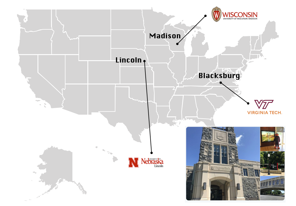 --- class: inverse, center, middle # Quantitative Genetics -- Analysis of complex or multifactorial traits -- All genes affect all traits - the question is by how much? -- Infinitesimal model -- Quasi-infinitesimal model, Oligogenic model --- # What is quantitative genetics? -- Population genetics - **Mathematics** is language of population genetics, **population genetics** is language of **evolution**. -- Quantitative genetics - **Statistics** is language of quantitative genetics, **quantitative genetics** is language of **complex trait genetics**. -- **Phenotypes** first in quantitative genetics In the era of genomics, phenotype is **king** <center> <iframe src="https://giphy.com/embed/9ADoZQgs0tyww" width="400" height="200" frameBorder="0" class="giphy-embed" allowFullScreen></iframe><p><a href="https://giphy.com/gifs/obama-awesome-statistics-9ADoZQgs0tyww">via GIPHY</a></p> </center> --- # Regression model Galton (1886). Regression towards mediocrity in hereditary stature "<img src="galton1886.png" width=600 height=380> --- # Complex traits <img src="phenotype-plant.png" width=800 height=530> --- # Genetic values Quantitative genetic model: `\begin{align*} \mathbf{y} &= \mathbf{g} + \boldsymbol{\epsilon} \\ \end{align*}` where `\(\mathbf{y}\)` is the vector of observed phenotypes, `\(\mathbf{g}\)` is the vector of genetic values, and `\(\boldsymbol{\epsilon}\)` is the vector of residuals. Example: | Animal ID | y | g | e | | ------------- |:-------------:| -----:|------| | 1 | 10 | ? | ? | | 2 | 7 | ? | ? | | 3 | 12 | ? | ? | --- # Genetic values Quantitative genetic model: `\begin{align*} \mathbf{y} &= \mathbf{g} + \boldsymbol{\epsilon} \\ \end{align*}` where `\(\mathbf{y}\)` is the vector of observed phenotypes, `\(\mathbf{g}\)` is the vector of genetic values, and `\(\boldsymbol{\epsilon}\)` is the vector of residuals. Example: | Animal ID | y | g | e | | ------------- |:-------------:| -----:|------| | 1 | 10 | 5 | 5 | | 2 | 7 | 6 | 1 | | 3 | 12 | 2 | 10 | -- Phenotypes can be observed and measured but genotypic and additive genetic effects cannot --- # Conventional Phenotyping 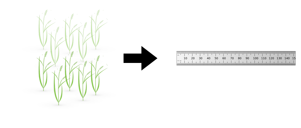 .pull-left[ - labor intensive - prone to measurement error ] .pull-right[ <iframe src="https://giphy.com/embed/Jk4ZT6R0OEUoM" width="500" height="160" frameBorder="0" class="giphy-embed" allowFullScreen></iframe><p><a href="https://giphy.com/gifs/Jk4ZT6R0OEUoM">via GIPHY</a></p> ] --- # Genomic information (e.g., SNPs) 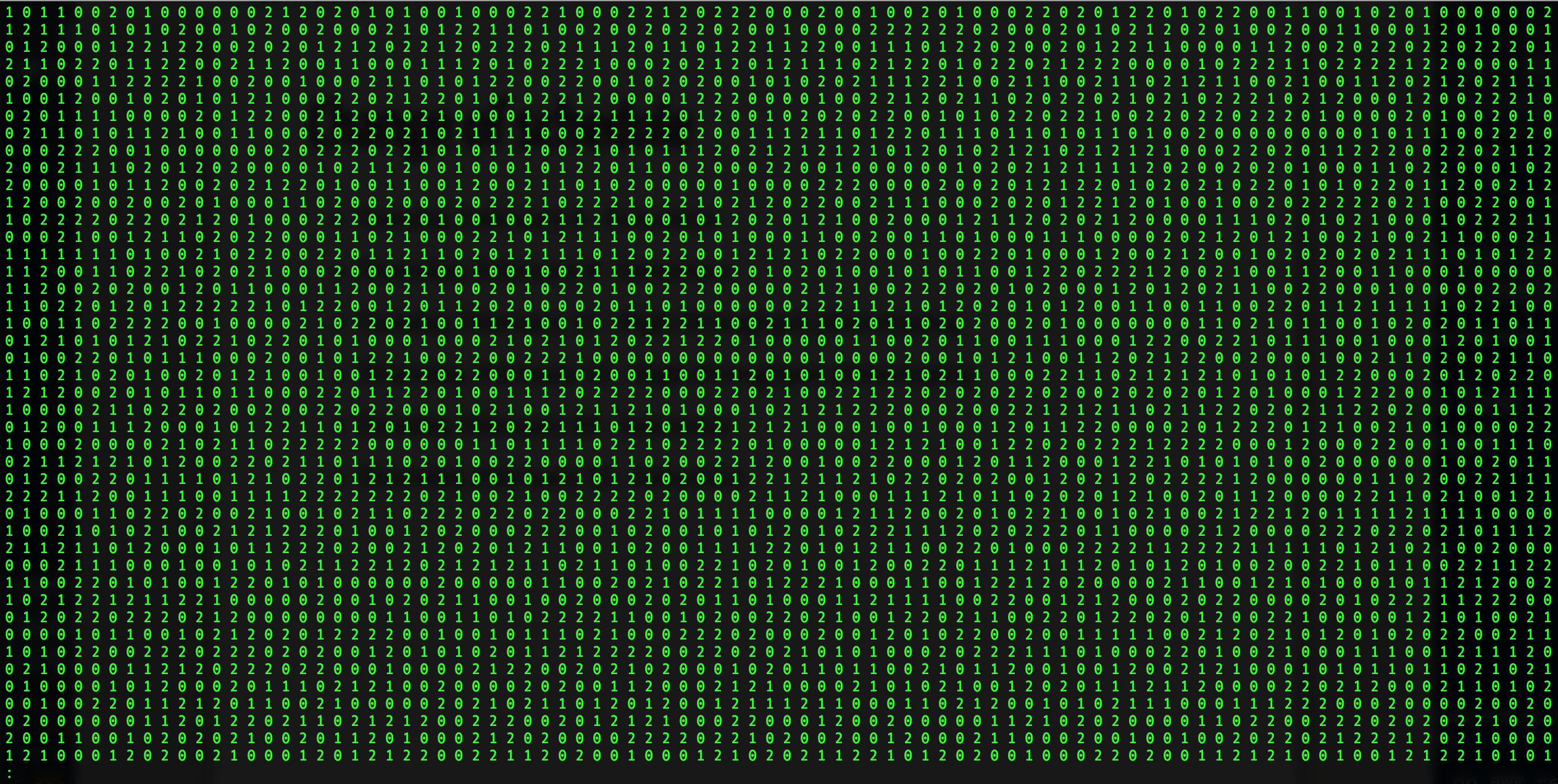 .center[Repeat of numbers 0, 1, and 2] --- # Quantitative genetics Connecting phenotypic data with genomic information<center> <div> <img src="plant.png" width=200 height=100> = <img src="SNPs.png" width=200 height=100> + error </div> </center> `\begin{align*} \mathbf{y} &= \mathbf{g} + \boldsymbol{\epsilon} \\ &\approx \mathbf{W}\mathbf{a} + \boldsymbol{\epsilon} \end{align*}` We approximate unknown `\(\mathbf{g}\)` with `\(\mathbf{Wa}\)`. `\begin{align*} \underbrace{\begin{bmatrix} y_1\\ y_2\\ \vdots \\ y_n\end{bmatrix}}_{n \times 1} &= \underbrace{\begin{bmatrix} w_{11} & w_{12} & \cdots & w_{1m} \\ w_{21} & w_{22} & \cdots & w_{2m} \\ \vdots & \vdots & \ddots & \vdots \\ w_{n1} & w_{n2} & \cdots & w_{nm} \end{bmatrix}}_{n \times m} \quad \underbrace{\begin{bmatrix} a_1\\ a_2\\ \vdots \\ a_m\end{bmatrix}}_{m \times 1} +\underbrace{\begin{bmatrix} \epsilon_1\\ \epsilon_2\\ \vdots \\ \epsilon_m\end{bmatrix}}_{n \times 1} \end{align*}` where `\(n\)` is the number of individuals (e.g., accessions) and `\(m\)` is the number of SNPs. --- # Precision agriculture using advanced technologies 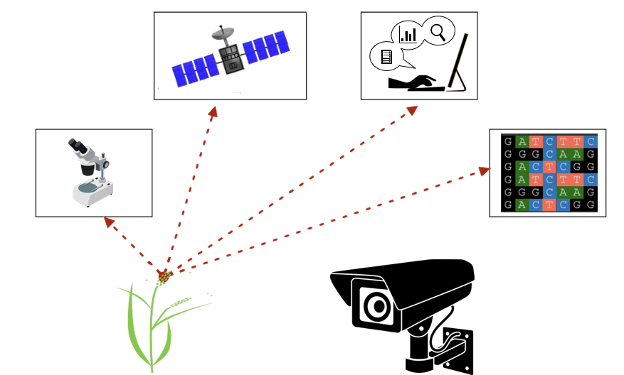 --- # Precision (digital) phenotyping 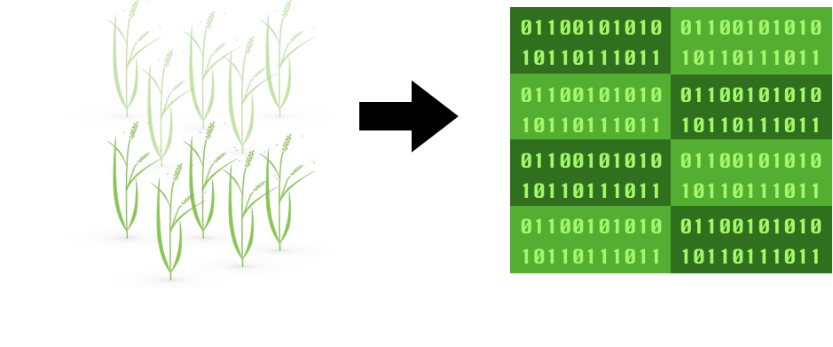 .pull-left[ - automated process - less labor intensive - less prone to measurement error ] .pull-right[ <iframe src="https://giphy.com/embed/wW95fEq09hOI8" width="400" height="160" frameBorder="0" class="giphy-embed" allowFullScreen></iframe><p><a href="https://giphy.com/gifs/chihuahua-funny-cute-wW95fEq09hOI8">via GIPHY</a></p> ] --- # Image phenotypes 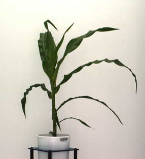 &nbsp; &nbsp;  .center[Image data] --- # Quantitative genetics Connecting image data with genomic information <center> <div> <img src="plant_01.png" width=100 height=100> = <img src="SNPs.png" width=100 height=100> + error </div> </center> `\begin{align*} \mathbf{y} &= \mathbf{g} + \boldsymbol{\epsilon} \\ &\approx \mathbf{W}\mathbf{a} + \boldsymbol{\epsilon} \end{align*}` We approximate unknown `\(\mathbf{g}\)` with `\(\mathbf{Wa}\)`. `\begin{align*} \underbrace{\begin{bmatrix} y_1\\ y_2\\ \vdots \\ y_n\end{bmatrix}}_{n \times 1} &= \underbrace{\begin{bmatrix} w_{11} & w_{12} & \cdots & w_{1m} \\ w_{21} & w_{22} & \cdots & w_{2m} \\ \vdots & \vdots & \ddots & \vdots \\ w_{n1} & w_{n2} & \cdots & w_{nm} \end{bmatrix}}_{n \times m} \quad \underbrace{\begin{bmatrix} a_1\\ a_2\\ \vdots \\ a_m\end{bmatrix}}_{m \times 1} +\underbrace{\begin{bmatrix} \epsilon_1\\ \epsilon_2\\ \vdots \\ \epsilon_m\end{bmatrix}}_{n \times 1} \end{align*}` where `\(n\)` is the number of individuals (e.g., accessions) and `\(m\)` is the number of SNPs. --- # Big in n or m? 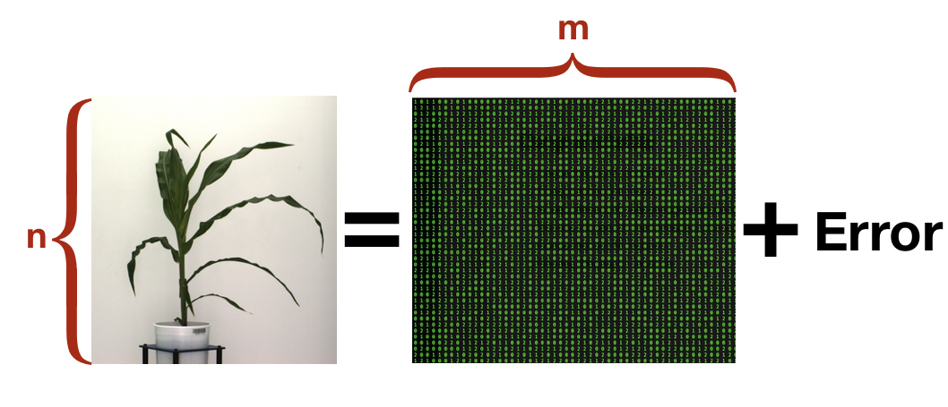 - `\(n\)`: number of individuals (records) - `\(m\)` number of SNPs (genetic markers) --- # Prediction vs. Inference Complex traits are controlled by large number of genes with small effects, and influenced by both genetics and environments - Inference (location) - average effects of allele substitution - Inference (variability) - variance component estimation - genomic heritability Combination of above two (e.g., estimate proportion of additive genetic variance explained by QTLs) - Prediction - genomic selection - prediction of yet-to-be observed phenotypes --- # Prediction vs. Inference <div align="center"> <img src="Lo2015PNAS.png" width=900 height=400> </div> * [http://www.pnas.org/content/112/45/13892.abstract ](http://www.pnas.org/content/112/45/13892.abstract ) --- # GWAS vs. Prediction  .right[[Wikimedia Commons](https://commons.wikimedia.org/wiki/File:Manhattan_Plot.png)]