Question 1

Read Whittaker et al. (2000) and summmarize the paper in 300 - 500 words.

Question 2

Recall that ridge estimates can be expressed as \(a^{ridge}_j = \frac{\sum^n_{i=1} w^2_{ij} }{\sum^n_{i=1} w^2_{ij} + \lambda} \times a^{ols}_{j}\). Create a centered genotype matrix Wc. Calculate the minor allele frequencies (MAF) and the amounts of shrinkage for all markers. Plot MAF on the X axis and the amounts of shrinkage on the Y axis. Interpret the figure you obtained. Use \(\lambda = 100\). Use the genotype matrix Wc.

Question 3

Fit a ridge regression using the glmnet R package. Create a scatterplot of marker effects when \(\lambda = 10\) (y-axix) and \(\lambda = 0.1\) (x-axis). Interpret the role of \(\lambda\) in the ridge regression. Use the variables y and W.

Question 4

Contrary to the ridge regression, the LASSO shrinks marker effects exactly equal to zero. Therefore, the LASSO can be used as a subset selection method.

aL <- glmnet(W, y, alpha = 1)
plot(aL$lambda, aL$df, ylab = "The number of nonzero markers", xlab = "Lambda")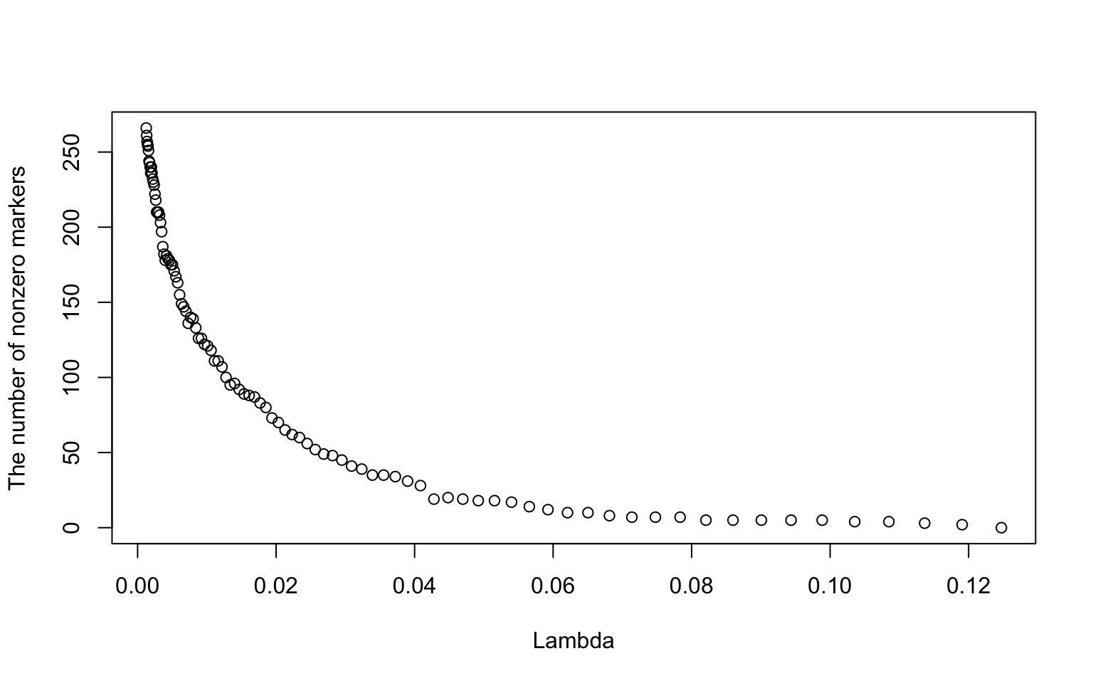

This figure shows the relationship between the sequence of \(\lambda\) values and the number of nonzero markers. Interpret the figure in the context of GWAS.