Bayesian Linear Regression

R script: myGibbs.txt
Literature 1: Mrode, R.A. 2005. Linear Models for the Prediction of Animal Breeding Values. CAB International, Oxon, UK.
Literature 2: Misztal, I. 2008. Computational Techniques in Animal Breeding. Course Notes. University of Georgia.

Given the components of MME, use Gibbs sampling. Consider the following univariate mixed linear model. In the Mixed Model Equation form: where 'A' is an additive relationship matrix and alpha is a ratio of the variance components. It can also be written as: Univariate Gibbs sampling can be performed by taking samples from following distribution.

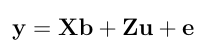
Here is a numerical application from Mrode (2005), example 12.1, which deals with the pre-weaning gain (WWG) of beef calves.

> # response
> y <- c(4.5,2.9,3.9,3.5,5.0)
>
> # pedigree
> s <- c(0,0,0,1,3,1,4,3)
> d <- c(0,0,0,0,2,2,5,6)
> Ainv <- quass(s,d)
> 
> # X matrix
> X <- matrix(c(1,0,0,1,1,0,1,1,0,0), nrow=5, ncol=2)
> X
     [,1] [,2]
[1,]    1    0
[2,]    0    1
[3,]    0    1
[4,]    1    0
[5,]    1    0
> # Z matrix
> z1 <- matrix(0, ncol=3, nrow=5)
> z2 <- matrix(c(1,0,0,0,0,0,1,0,0,0,0,0,1,0,0,0,0,0,1,0,0,0,0,0,1), ncol=5)
> Z <- cbind(z1,z2)
> Z
     [,1] [,2] [,3] [,4] [,5] [,6] [,7] [,8]
[1,]    0    0    0    1    0    0    0    0
[2,]    0    0    0    0    1    0    0    0
[3,]    0    0    0    0    0    1    0    0
[4,]    0    0    0    0    0    0    1    0
[5,]    0    0    0    0    0    0    0    1

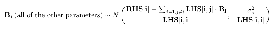
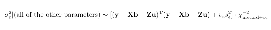
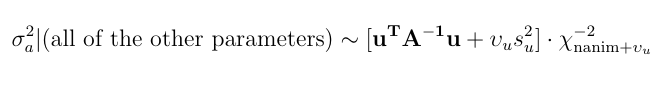
Set the initials of B (b and u) to zero, the environmental variance to 40, the additive genetic variance to 20 and assume "naive" ignorance improper priors for the variance components such that ve = va = 0 and s2e = s2e = 0

> inits <- c(0,0,0,0,0,0,0,0,0,0)
> varE <- 40
> varA <- 20
> ve <- 0
> va <- 0
> s2e <- 0
> s2a <- 0

Further, allow 2000 "burnin" samples. Then collect 5000 samples after the burnin period. Define the disp option as TRUE.

> burnin <- 2000
> N <- 5000
> disp <- TRUE

To get the complete result, let's run myGibbs function.

> myGibbs(Ainv, y, X, Z, N, burnin, inits, varE, varA, ve, va, s2e, s2a, disp)

iteration  1 
varA  27.90349 
varE  9.830295 

iteration  2 
varA  27.62676 
varE  6.469905 

iteration  3 
varA  3.537537 
varE  1.264450 

     .
     .
     .
     snip
     .
     .
     .

iteration  6998 
varA  0.08454485 
varE  0.2756133 

iteration  6999 
varA  0.3397200 
varE  0.5079951 

iteration  7000 
varA  0.6410488 
varE  0.336344 

$`Solutions`
 [1]  4.42481745  3.46324977  0.04799799 -0.07124684 -0.06597394 -0.05571167
 [7] -0.23979331  0.11705991 -0.30874805  0.12379153

$`Variance Components`
[1] 1.269034 2.032178

Solutions[1] and Solutionss[2] are sex effects. Prediction[3] through Prediction[10] are predicted breeding values. The first variance component is an estimate of the additive genetic variance and the second one is an estimate of the envirommental variance.

Bayesian Linear Regression

List

Univariate Gibbs Sampler