Back

Iterative Methods for Solving Mixed Model Equations (MME)

List

• Jocobi Over Relaxation
• Successive Over Relaxation

Jacobi Over Relaxation

• R script: jor.txt
• Literature 1: Mrode, R.A. 2005. Linear Models for the Prediction of Animal Breeding Values. CAB International, Oxon, UK.
• Literature 2: Misztal, I. 2008. Computational Techniques in Animal Breeding. Course Notes. University of Georgia.

1. Given the MME, iteratively solve for the solutions by Jocobi Over Relaxation. Consider the following univariate mixed linear model. In the Mixed Model Equation form: where 'A' is an additive relationship matrix and alpha is a ratio of the variance components. It can also be written as: The left hand side can be decomposed into: where D is the diagonal matrix and R is the remainder. The (t + 1)th solutions are obtained using the equation: where w is the diagonal matrix of relaxation factor.
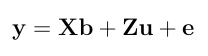
2. Here is a numerical application from Mrode (2005), example 3.1, concerning the pre-weaning gain (WWG) of beef calves.

   > # response
   > y <- c(4.5,2.9,3.9,3.5,5.0)
   >
   > # pedigree
   > s <- c(0,0,0,1,3,1,4,3)
   > d <- c(0,0,0,0,2,2,5,6)
   > Ainv <- quass(s,d)
   >
   > # variance component ratio
   > vcr = 40/20
   > 
   > # X matrix
   > X <- matrix(c(1,0,0,1,1,0,1,1,0,0), nrow=5, ncol=2)
   > X
        [,1] [,2]
   [1,]    1    0
   [2,]    0    1
   [3,]    0    1
   [4,]    1    0
   [5,]    1    0
   
   > # Z matrix
   > z1 <- matrix(0, ncol=3, nrow=5)
   > z2 <- matrix(c(1,0,0,0,0,0,1,0,0,0,0,0,1,0,0,0,0,0,1,0,0,0,0,0,1), ncol=5)
   > Z <- cbind(z1,z2)
   > Z
        [,1] [,2] [,3] [,4] [,5] [,6] [,7] [,8]
   [1,]    0    0    0    1    0    0    0    0
   [2,]    0    0    0    0    1    0    0    0
   [3,]    0    0    0    0    0    1    0    0
   [4,]    0    0    0    0    0    0    1    0
   [5,]    0    0    0    0    0    0    0    1
   
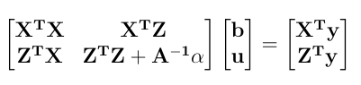
   > Xpy <- t(X)%*%y
   > Zpy <- t(Z)%*%y
   > XpX <- t(X)%*% X
   > XpZ <- t(X)%*%Z
   > ZpX <- t(Z)%*%X
   > ZpZ <- t(Z)%*%Z
   > 
   > LHS <- rbind( cbind(XpX, XpZ), cbind(ZpX, ZpZ+Ainv*vcr))
   > RHS <- c(Xpy, Zpy)
   

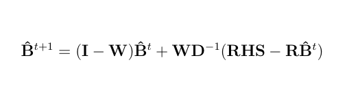
   The relaxation factor has been chosen as 1.0 for the fixed effects and 0.8 for the random effects. Initial values included the mean yield for fixed effects. For animals with phenotypic records, initial values were the deviation of yields from the mean yield of their respective fixed effects and zero for animals without phenotypic records.

   > inits <- c(4.333,3.400,0,0,0,0.167,-0.5,0.5,-0.833,0.667)
   > w <- c(1,1,rep(0.8,8))
   > disp = FALSE
   

3. The final solutions were:

   > jor(LHS, RHS, inits, w, disp=FALSE)
   
   Final solutions after 18 th iteration              [,1]
    [1,]  4.357884994
    [2,]  3.403872956
    [3,]  0.099030310
    [4,] -0.018384432
    [5,] -0.041024426
    [6,] -0.008047532
    [7,] -0.185301976
    [8,]  0.177676221
    [9,] -0.248927431
   [10,]  0.183120263
   

Successive Over Relaxation

• R script: sor.txt
• Literature 1: Mrode, R.A. 2005. Linear Models for the Prediction of Animal Breeding Values. CAB International, Oxon, UK.
• Literature 2: Misztal, I. 2008. Computational Techniques in Animal Breeding. Course Notes. University of Georgia.

1. Given the MME, iteratively solve for the solutions by Successive Over Relaxation. SOR works like JOR except that solutions which already have been computed are used immediately at each time. Applying SOR to the same data as above without relaxation factor (Gauss Seidel method in this case) gives:

   > w2 <- rep(1,10)
   > sor(LHS, RHS, inits, w2, disp=FALSE)
   
   Final solutions after 11 th iteration              [,1]
    [1,]  4.359129262
    [2,]  3.405185500
    [3,]  0.097986927
    [4,] -0.019280834
    [5,] -0.041467395
    [6,] -0.009058115
    [7,] -0.186312311
    [8,]  0.176258201
    [9,] -0.249974023
   [10,]  0.182090470