Back

Variance Components Estimation

List

• REML (Newton Raphson)
• REML (Fisher's Scoring)
• REML (Average Information)
• REML (EM Algorithm)

REML (Newton Raphson)

• R script: nrReml.txt
• Literature 1: Tsuruta, S. 2006. Estimation of Variance Components in Animal Breeding. The University of Georgia.
• Literature 2: Mrode, R.A. 2005. Linear Models for the Prediction of Animal Breeding Values. CAB International, Oxon, UK.

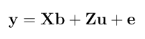
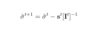
1. Given the components of the MME, estimate variance components by REML using Newton Raphson framework. Consider the following univariate mixed linear model. The Newton Raphson method works as the next equation and repeat this process untill it achives convergence. 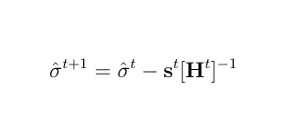where s is the score vector and H is the Hessian matrix for the log-likelihood of variance components.
2. Here is a numerical application where the data is from Mrode (2005), example 11.6, concerning the pre-weaning gain (WWG) of beef calves.

> # response
> y <- c(2.6,0.1,1.0,3.0,1.0)
>
> # pedigree
> s <- c(0,0,0,1,3,1,4,3)
> d <- c(0,0,0,0,2,2,5,6)
> A <- createA(s,d)
>
> # X matrix
> X <- matrix(c(1,0,0,1,1,0,1,1,0,0), nrow=5, ncol=2)
> X
     [,1] [,2]
[1,]    1    0
[2,]    0    1
[3,]    0    1
[4,]    1    0
[5,]    1    0
>
> # Z matrix
> z1 <- matrix(0, ncol=3, nrow=5)
> z2 <- matrix(c(1,0,0,0,0,0,1,0,0,0,0,0,1,0,0,0,0,0,1,0,0,0,0,0,1), ncol=5)
> Z <- cbind(z1,z2)
> Z
     [,1] [,2] [,3] [,4] [,5] [,6] [,7] [,8]
[1,]    0    0    0    1    0    0    0    0
[2,]    0    0    0    0    1    0    0    0
[3,]    0    0    0    0    0    1    0    0
[4,]    0    0    0    0    0    0    1    0
[5,]    0    0    0    0    0    0    0    1

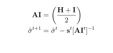
In this particular design, the Hessian Matrix is going to be singular and unable to take inverse. Thus, we will add one data point.

> y <- c(y, 2.0)
> addX <- matrix(c(0,1), ncol=2)
> X <- rbind(X,addX)
> X
     [,1] [,2]
[1,]    1    0
[2,]    0    1
[3,]    0    1
[4,]    1    0
[5,]    1    0
[6,]    0    1
> addZ <- matrix(c(0,0,0,0,0,1,0,0), ncol=8)
> Z <- rbind(Z, addZ)
> Z
     [,1] [,2] [,3] [,4] [,5] [,6] [,7] [,8]
[1,]    0    0    0    1    0    0    0    0
[2,]    0    0    0    0    1    0    0    0
[3,]    0    0    0    0    0    1    0    0
[4,]    0    0    0    0    0    0    1    0
[5,]    0    0    0    0    0    0    0    1
[6,]    0    0    0    0    0    1    0    0

Our initials for the variance components will be:

> initE <- 0.4
> initU <- 0.2
> disp <- TRUE

After 18 iterations, Newton Raphson gives following estimates.

> nrReml(A, y, X, Z, initE, initU, disp)

iteration  1 
sig2U 0.3055028 
sig2E 0.4688081 

iteration  2 
sig2U 0.4567926 
sig2E 0.4962741 

iteration  3 
sig2U 0.6235681 
sig2E 0.4954533 

     .
     .
    snip
     .
     .

iteration  16 
sig2U 1.128275 
sig2E 0.4891807 

iteration  17 
sig2U 1.128592 
sig2E 0.489179 

iteration  18 
sig2U 1.128775 
sig2E 0.489178 

$sigma2U
[1] 1.128775

$sigma2E
[1] 0.489178

REML (Fisher's Scoring )

• R script: fsReml.txt
• Literature 1: Tsuruta, S. 2006. Estimation of Variance Components in Animal Breeding. The University of Georgia.
• Literature 2: Mrode, R.A. 2005. Linear Models for the Prediction of Animal Breeding Values. CAB International, Oxon, UK.

1. Given the components of the MME, estimate variance components by REML using Fisher's Scoring framework. Consider the following univariate mixed linear model. In Fisher Scoring, the Hessian matrix is replaced by Fisher's information matrix I.
2. Applying Fisher's Scoring to the same data used in Newton Raphson example gives:

   > fsReml(A, y, X, Z, initE, initU, disp)
   
   iteration  1 
   sig2U 3.125955 
   sig2E 0.4964242 
   
   iteration  2 
   sig2U 2.872239 
   sig2E 0.4960792 
   
   iteration  3 
   sig2U 2.620172 
   sig2E 0.4957264 
   
        .
        .
       snip
        .
        .
   
   iteration  20 
   sig2U 1.129177 
   sig2E 0.4891795 
   
   iteration  21 
   sig2U 1.129097 
   sig2E 0.489178 
   
   iteration  22 
   sig2U 1.129058 
   sig2E 0.4891773 
   
   $sigma2U
   [1] 1.129058
   
   $sigma2E
   [1] 0.4891773
   

REML (Average Information )

• R script: aiReml.txt
• Literature 1: Tsuruta, S. 2006. Estimation of Variance Components in Animal Breeding. The University of Georgia.
• Literature 2: Mrode, R.A. 2005. Linear Models for the Prediction of Animal Breeding Values. CAB International, Oxon, UK.

1. Given the components of MME, estimate variance components by REML in the Average Information framework. Consider the following univariate mixed linear model. Average Information REML uses the average value of the Hessian matrix and Fisher's information matrix I.
2. Applying AI-REML on the same data used in Newton Raphson gives:

   > aiReml(A, y, X, Z, initE, initU, disp)
   
   iteration  1 
   sig2U 0.2557512 
   sig2E 0.6310165 
   
   iteration  2 
   sig2U 0.3762888 
   sig2E 0.7520789 
   
   iteration  3 
   sig2U 0.6048932 
   sig2E 0.6404164 
   
        .
        .
       snip
        .
        .
   
   iteration  18 
   sig2U 1.128901 
   sig2E 0.4891792 
   
   iteration  19 
   sig2U 1.128955 
   sig2E 0.4891781 
   
   iteration  20 
   sig2U 1.128985 
   sig2E 0.4891774 
   
   $sigma2U
   [1] 1.128985
   
   $sigma2E
   [1] 0.4891774
   

REML (EM Algorithm)

• R script: emReml.txt
• Literature 1: Suzuki, M. 2007. Applied Animal Breeding & Genetics. Course Notes. Obihiro University of Agriculture and Veterinary Medicine.
• Literature 2: Mrode, R.A. 2005. Linear Models for the Prediction of Animal Breeding Values. CAB International, Oxon, UK.

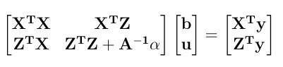
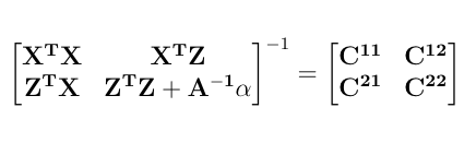
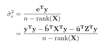
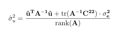
1. Given the components of MME, estimate variance components by the EM Algorithm. Consider the following univariate mixed linear model. In the Mixed Model Equation form: Further, let the inverse of the left hand side be: The EM Algorithm can be implemented by following successive iterations.
2. An example is taken from Mrode (2005), 11.6, concerning the pre-weaning gain (WWG) of beef calves.

   > # response
   > y <- c(2.6,0.1,1.0,3.0,1.0)
   >
   > # pedigree
   > s <- c(0,0,0,1,3,1,4,3)
   > d <- c(0,0,0,0,2,2,5,6)
   > Ainv <- quass(s,d)
   >
   > # X matrix
   > X <- matrix(c(1,0,0,1,1,0,1,1,0,0), nrow=5, ncol=2)
   > X
        [,1] [,2]
   [1,]    1    0
   [2,]    0    1
   [3,]    0    1
   [4,]    1    0
   [5,]    1    0
   >
   > # Z matrix
   > z1 <- matrix(0, ncol=3, nrow=5)
   > z2 <- matrix(c(1,0,0,0,0,0,1,0,0,0,0,0,1,0,0,0,0,0,1,0,0,0,0,0,1), ncol=5)
   > Z <- cbind(z1,z2)
   > Z
        [,1] [,2] [,3] [,4] [,5] [,6] [,7] [,8]
   [1,]    0    0    0    1    0    0    0    0
   [2,]    0    0    0    0    1    0    0    0
   [3,]    0    0    0    0    0    1    0    0
   [4,]    0    0    0    0    0    0    1    0
   [5,]    0    0    0    0    0    0    0    1
   

   As in Mrode (2005), set the initial values for the residual variance to 0.4 and set the additive variance to 0.2.

   > # initial variance components
   > initE <- 0.4
   > initU <- 0.2
   >
   > disp = TRUE
   

   The EM algorithm gives the following estimates after 906 iterations.

   > emReml(Ainv, y, X, Z, initE, initU, disp)
   
   iteration  1 
   sig2E 0.6425753 
   sig2U 0.2124631 
   
   iteration  2 
   sig2E 0.7061095 
   sig2U 0.2145396 
   
   iteration  3 
   sig2E 0.7174604 
   sig2U 0.2153153 
   
        .
        .
       snip
        .
        .
   
   iteration  904 
   sig2E 0.4848573 
   sig2U 0.5493628 
   
   iteration  905 
   sig2E 0.4848473 
   sig2U 0.5493777 
   
   iteration  906 
   sig2E 0.4848373 
   sig2U 0.5493925 
   
   $sigma2E
             [,1]
   [1,] 0.4848373
   
   $sigma2U
             [,1]
   [1,] 0.5493925